Monte Carlo arithmetic and stochastic rounding
Randomized arithmetic is specified by its probability law and instrumented scope. Distance-weighted stochastic rounding, equal-probability endpoint rounding, and Monte Carlo arithmetic can induce different means and dispersions. This guide derives those distinctions before examining a reproducible fixed-grid experiment.
Distance-weighted stochastic rounding
Let \(a<b\) be adjacent representable values enclosing an exact result \(x\). Ideal stochastic rounding selects
\[\operatorname{SR}(x)= \begin{cases} a,&\text{with probability }(b-x)/(b-a),\\ b,&\text{with probability }(x-a)/(b-a). \end{cases}\]Representable values are left unchanged. For an interior point, direct calculation gives
\[\mathbb E[\operatorname{SR}(x)\mid x]=x, \qquad \operatorname{Var}(\operatorname{SR}(x)\mid x)=(x-a)(b-x).\]Thus the local rounding error has conditional mean zero under ideal probabilities. Its variance is largest halfway between endpoints and vanishes at either endpoint. This local property does not, by itself, prove that the output of a nonlinear program is unbiased: nonlinear transformations and branch selection require their own analysis.
Connolly, Higham, and Mary (2021) develop probabilistic backward-error analysis under suitable mean-independence assumptions. Finite random-bit implementations require additional analysis; El Arar and colleagues (2025) study the resulting bias. The ideal formula should not be assumed to describe every implementation exactly.
Equal endpoint probabilities and Monte Carlo arithmetic
For a nonrepresentable interior result, selecting \(a\) and \(b\) with probability one half gives mean \((a+b)/2\). The local bias relative to \(x\) is then
\[\mathbb E[\operatorname{RR}(x)-x\mid x]=(a+b)/2-x.\]It vanishes at the midpoint, but generally differs from ideal distance-weighted SR. Terms such as “random rounding” are used for several implementations; report the probability law rather than relying on the name alone.
Monte Carlo arithmetic introduces arithmetic perturbations at a chosen virtual precision. A simplified centered perturbation at a nonzero normalized value can be written
\[\widetilde x=x+\Delta_t(x)\xi,\qquad \Delta_t(x)=2^{\lfloor\log_2|x|\rfloor-t+1},\qquad \xi\sim\mathcal U(-1/2,1/2).\]Here \(t\) is the significand precision and \(\Delta_t\) is the spacing of its local binary grid. An implementation also specifies whether perturbations affect operands, results, or both, and how exact values and exceptional cases are handled. This expression illustrates a model; it is not a complete specification of a particular backend. See the Verificarlo backend documentation.
A fixed-grid summation experiment
The example script sums the exact increment \(1/40\) 400 times, rounding after every addition to multiples of \(1/8\). Its exact real-arithmetic sum is 10. Intermediate values are Python Fraction objects, and SR uses exact integer sampling to implement its rational endpoint probabilities.
At every step, the increment is one fifth of the grid spacing. Nearest rounding stagnates at zero. SR advances one grid cell with probability \(1/5\), so its final result has mean 10 and standard deviation 1. Equal endpoint probabilities instead advance with probability \(1/2\), producing mean 25 and standard deviation 1.25. These conclusions follow from a binomial sum on this fixed grid; floating-point grids have varying spacing and require separate analysis.
python3 stochastic_rounding.py
Download the script first. It requires only the standard library. For 1,000 repetitions with seeds 7–1006, the recorded run produced:
| Rounding rule | Sample mean | Sample standard deviation |
|---|---|---|
| Nearest | 0 | 0 |
| Distance-weighted SR | 10.008625 | 0.984348 |
| Equal endpoint probabilities | 25.010625 | 1.221867 |
The script checks the sample means against six-standard-error intervals around the analytical expectations. The finite samples do not establish the probability laws; those were derived above.
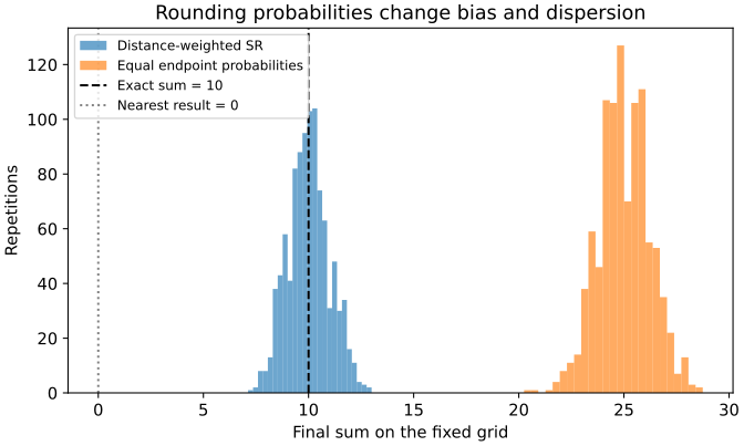
Figure: results generated by the fixed-grid experiment. This is neither a hardware benchmark nor a simulation of a complete MCA backend.
Regenerate the figure with Matplotlib 3.11.2:
python3 stochastic_rounding.py --plot stochastic-rounding.svg
The recorded environment was Python 3.12.3, Matplotlib 3.11.2, and NumPy 2.5.3 on Linux x86_64. The arithmetic and random sampling use the standard library.
Experimental interpretation
Choose the perturbation model to match the question: precision requirements, sensitivity to roundoff, or numerical variation across a defined execution scope. Record virtual precision, rounding law, backend revision, seeds, and library coverage. Changing arithmetic seeds while also changing data order or model initialization confounds the sources of variation.
Fuzzy PyTorch evaluates stochastic arithmetic in deep-learning computations. Its published study compares specific implementations and workloads; those performance comparisons cannot be inferred from the fixed-grid example.
References
- Connolly, Higham, and Mary (2021), Stochastic rounding and its probabilistic backward error analysis.
- El Arar, Fasi, Filip, and Mikaitis (2025), Probabilistic error analysis of limited-precision stochastic rounding.
- Reviewed Verificarlo backends.
- Python conditioning and stability example.